Is Deep Better in Extreme Temperature Forecasting?
Article information
Abstract
최근 들어서 인공신경망을 이용한 딥러닝이 강우, 풍속, 온도 등의 높은 비선형성과 복잡성을 가진 여러 기상현상을 예측하는데 널리 이용되어지고 있다. 하지만 실제적인 딥러닝이 그만큼의 성능을 발휘하는지에 대한 중요한 연구들은 실제로 많이 이루어지지 못하고 있다. 따라서 본 연구에서는 하나의 은닉층을 바탕으로 한 얕은 층의 모형과 여러 은닉층을 가진 깊은 은닉층의 모형에 대해서 비교 평가하였다. 자료는 한국의 5개 기상관측지점을 대상으로 1975-2015년의 일최고기온을 바탕으로 수행되어졌다. 각각의 모형은 겨울, 봄, 여름, 가을 자료의 1일단위 예측하는데 적용되었다. 이와 더불어, 모델의 성능과 효율성이 RMSE를 통해 평가되었고, 유전알고리즘이 최상의 네트워크구조를 찾는데 사용되었다. 전체적으로, 한 개의 은닉층을 가진 모형이 다수의 은닉층을 가진 모델보다 더 좋은 성능을 가지는 특징을 보여 주었다.
Trans Abstract
In recent years, the application of deep learning based on artificial neural networks (ANNs) to forecast highly non-linear and complex weather phenomena, such as rainfall, wind speed, and temperature, has become an attractive pursuit in the field of environmental sciences. However, the critical research addressing the question of whether or not a deep learning network can perform better has not been completed. The current study conducted a systematic comparison of a one-hidden-layer (shallow) network and a multiple-hidden-layer (deep) network in maximum temperature forecasting Datasets of daily maximum temperature at five stations in South Korea, spanning the years 1976 to 2015, were used for training and testing the different-architecture models, respectively. With each model, one-day-ahead forecasting was made for the winter, spring, summer, and autumn seasons. Moreover, the performance and effectiveness of the models were then assessed by the root mean square error (RMSE). In addition, a genetic algorithm was applied to select the optimal network architecture. Finally, the empirical results indicated that the ANN model with one hidden layer, compared with the case of multiple-hidden-layer networks, produced the most accurate forecasts.
1. Introduction
The Earth’s climate has changed considerably over the past century due to natural processes and human activities, which has the ability to change extreme intensity and frequency. More severe climate change can trigger drastic effects with unexpected consequences. Therefore, climate extreme projection is important information required to evaluate the effect of future climate change on human beings and on the environment. Such information also enables to help all countries in the world to build long‐term strategies to mitigate and adapt effectively to climate change. The process of climate change, especially the changing of temperature and rainfall, is the most significant problem in environmental sciences.
Temperature‐based forecasting is essential for agriculture, water resources, and human activities. The present study, therefore, focused on daily maximum forecasting. In order to predict the weather in an effective way, in this study, we have suggested a weather forecasting model using Artificial Neural Network (ANN). In ANN, there are an input layer, an output layer, and some hidden layers. The number of neurons per layer and the number of hidden layers determine the ability of the networks to produce accurate results for a specific set of data.
In latest years, ANNs have been extensively researched and effectively implemented in multiple areas, such as hydrology and water resources because of the capability of handling high non‐linearity and huge data (Hung et al., 2009). Several works have been done and different ANN models have been tested. Fahimi Nezhad et al. (2019) considered and predicted Tehran maximum temperature in winter using five different neural network models and found that the model with three neurons in the input layers and nine neurons in the hidden layer was the most accurate model with the least error and the most correlation coefficient.
In another research, Smith et al. (2007) developed an ANN model to predicted air temperature for one to 12 hours ahead. Furthermore, a study about rainfall prediction based on past observation using ANN and autoregressive integrated moving average (ARIMA) has been implemented by Somvanshi et al. (2006). The results showed that the ANN model, which outperforms the ARIMA model, can be a suitable forecasting tool to predict the rainfall.
The word “deep” in deep learning shows that such an artificial neural network (ANN) includes more layers than the “shallow” (i.e., one‐hidden‐layer) ones. In some previous literature, it is shown that such deep architecture can provide higher learning ability and better generalization compared to shallow structures (Sagheer and Kotb, 2019). Chen and Chang (2009) applied evolutionary artificial neural networks to forecast 10‐day reservoir inflows. The results revealed that the optimal architecture of model using three hidden layers produced better results compared to one‐hidden‐layer as well as autoregressive (AR) and autoregressive moving average exogenous (ARMAX) models.
However, is a deep network better than a shallow one in forecasting maximum temperature? To the knowledge of the authors, no work has been studied to conduct fair and systematic comparisons of single (shallow) and multiple‐hidden‐layer (deep) networks in this problem. Therefore, in the present study, we investigated a systematic comparison of shallow and deep networks in forecasting one‐day‐ahead maximum temperature by conducting an extensive multiple‐case study.
The rest of the paper has been organized as follows. Section 2 is dedicated to an explanation of the data used for experiments. The methodology based on Artificial Neural Networks (ANNs) for one‐day‐ahead maximum temperature forecasting is proposed in Section 3. Then, the obtained results are described in Section 4. Finally, the conclusion is made in Section 5.
2. Data description
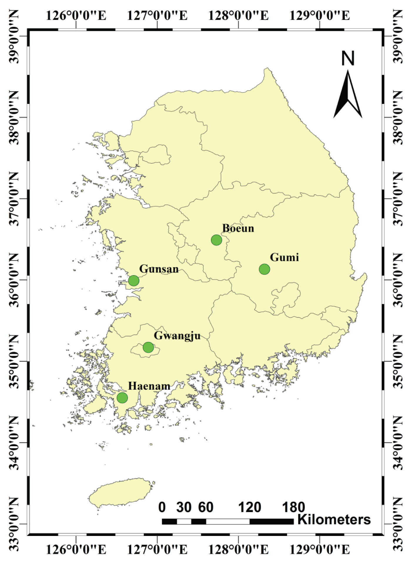
The data recorded at five stations in South Korea, namely Gunsan, Gumi, Boeun, Gwangju, and Haenam, were collected to develop and analyze the forecasting models. Locations of five stations are shown in Fig. 1. The datasets in five stations consist of daily maximum temperature from 1976 to 2015. To examine the seasonal variations, the data were split into four seasons, which are winter (December‐February), spring (March‐May), summer (June‐August) and autumn (September‐ November).
The designing models start with one hidden layer and then two and three hidden layers to compare the performance of shallow and deep networks and obtain the best network for forecasting problem. Because changes in the number of the hidden layer neurons can have an important effect on network performance precision, the number of neurons has been changed from 1 to 20 to determine the best number of hidden neurons. Inputs to the model were daily maximum temperature data (at time t) and past daily maximum temperature with sevendaily lag times i.e., from (t-6) to (t), while the output is the temperature of the next day (t+1). Then, the dataset was standardized for each season as Equation (10):
where: x't and xt are the original and transformed explanatory variables, respectively; mx and sx are the mean and standard deviation of the original variable x, respectively.
Neural networks generally provide improved performance with the standardized data. Using original data as the input to the neural network may cause a convergence problem. The data of daily maximum temperature were used to train and test the ANN model. One‐day‐ahead forecasts are made for the winter, spring, summer, and autumn seasons in each station.
3. Methodology
3.1 Artificial Neural Network (ANN) model
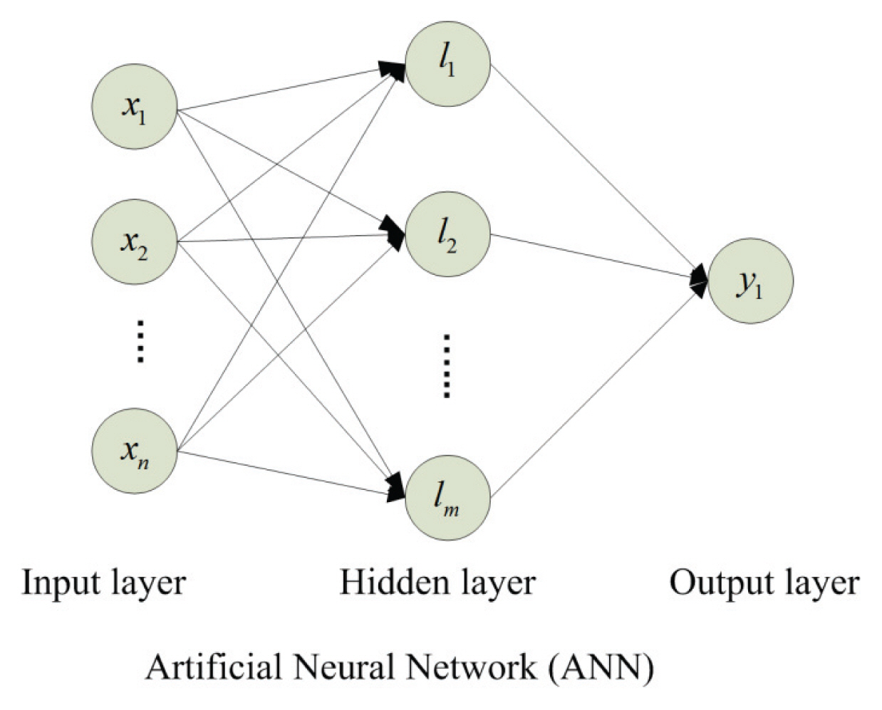
ANN is a powerful tool for modeling data that enables to capture and generate the complex relationship between input and output. The fundamental and important elements of an ANN are neurons which can obtain inputs, process them and generate the appropriate outputs like the natural neuron in the human brain. An ANN consists of three layers, which are connected to each other, as illustrated in Fig. 2. The first layer called an input layer has a function to receive input information while the last layer, which generates results for a specified problem, is called an output layer. Between output and input layers are one or more hidden layers. Information is transferred through the connected nodes in different layers. The relationship between the output yt and the inputs (xt-1;xt-2;…xt-i) can be calculated by the following mathematical equation:
where, wj and wi are the connection weights; G1 and G2 are activation function while bi and bj are the bias of each layer.
In this study, the tanh function is used as an activation function of the input and hidden neurons while a linear function is allocated as an activation function of output neurons in models. The tanh function is defined as:
The use of tanh function is to help the model capture complex and nonlinear phenomena. Meanwhile, the liner function is used in the output layer to produce an output signal corresponding to the input in case of the regression problem. The ANN’s primary parameters are the weights. The procedures of estimating these parameters are trained in the network where optimal weights are calculated by minimizing an objective function.
3.2 Model development
The dataset was divided into three sets including training, validation, and test sets. The training set was used to fit the model; the validation data used to find the optimal network architecture and then the testing data used to check the network performance. In this study, 80% of the data was used as the training set, while the rest 20% was selected as the test set. Furthermore, 20% of the training set was chosen as the validation set to validate the efficiency of the model. We used the training set to train ANN models and then measured the root mean square error (RMSE) of predicted values corresponding to the validation set.
In the ANN’s training phase, we use the Genetic Algorithm (GA) to find the optimal hyper‐parameters (number of hidden neurons and number of epochs) for the proposed model by choosing the smallest RMSE on the validation set. We applied the GA using Distributed Evolutionary Algorithms in Python (DEAP) library (Fortin et al., 2012). Lastly, we fit the model with the selected hyperparameter value to both the training and validation data and make predictions corresponding to the test data. Genetic parameters, such as crossover rate, mutation rate, and population size, may affect the result in order to achieve the best option for the problem. In the current study, we use a population size of 10, crossover and mutation rate will be 0.4 and 0.1, respectively. The number of epochs from 20 to 300 will be tested. The number of generations is assigned as 10 as a terminated condition.
To estimate the prediction accuracy and evaluate the performance of the forecast, the root mean square error (RMSE) and the squared coefficient of correlation (R2) were used. The indices can be calculated as follows:
where, xt is the current true value,
The optimal model is the one that has the lowest RMSE and the smaller the value of RMSE, the closer the predicted values by the model to the true values.
4. Results
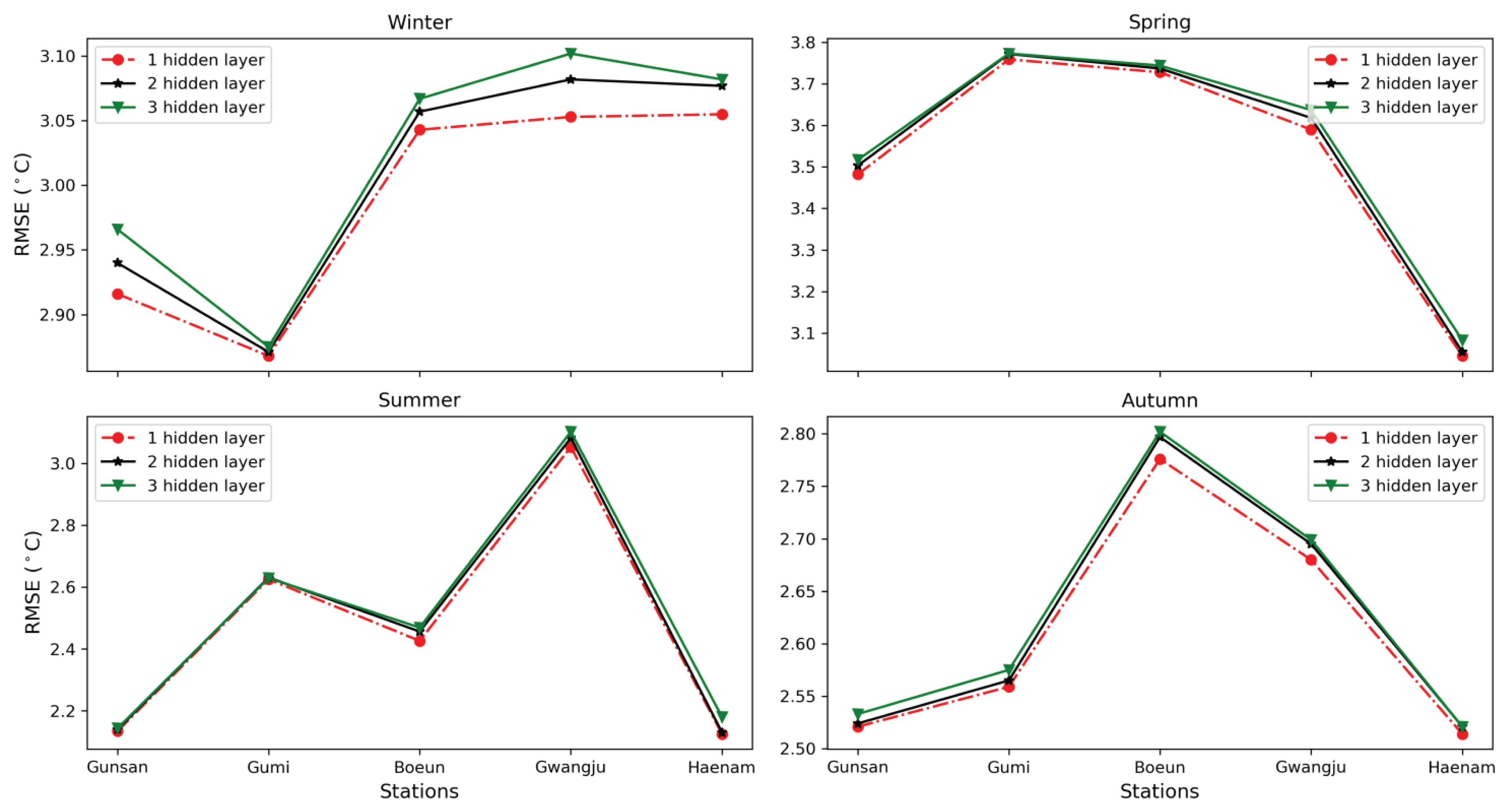
In this section, we present the results of our multiple‐case study. The performance criterion, RMSE, was calculated using the test data to find the optimal number of the hidden nodes. It can be observed from Fig. 3 that the best results of ANN for every season were achieved using a one‐hidden‐layer variant in all five stations. Especially, the single hidden layer model generated considerable lower values of RMSE than multiple hidden layers for winter in four stations which were Gunsan, Boeun, Gwangju and Haenam stations. Comparison of single hidden layer and multiple hidden layers for the forecasting of maximum temperature in four seasons in Gunsan, Boeun, Gumi, Gwangju, and Haenam stations are shown in Tables 1~5, respectively. Notably, the results shown in all tables represent the performance of the model in testing data. Shown in each row of tables is the result of the best network of a given hidden layer.

Root Mean Square Error Corresponding to Different Number of Hidden Layers for Winter, Spring, Summer, and Autumn in Five Stations
For example, as indicated in Table 1 the best one‐hiddenlayer ANN in Gunsan station in winter was the one which consisted of 8 hidden neurons. Similarly, the best 2‐hiddenlayer ANN was the one which consisted of 13 and 12 hidden neurons, and so on. It is clear that one‐hidden‐layer ANN model presented the best performance for winter, spring, summer, and autumn with the values of 2.916°C, 3.482°C, 2.134°C, and 2.521°C for RMSE, respectively.
In general, it can be noticed that the maximum temperature for one‐day‐ahead forecasts in summer was predicted with the lowest RMSE values of 2.134°C, 2.426°C, 2.326°C, and 2.125°C in Gunsan, Boeun, Gwangju, and Haenam, respectively. However, in Gumi station, the autumn season had the lowest RMSE of 2.559°C. On the other hand, the obtained results from changing the number of the designed network hidden layers showed that the rising of the hidden layer’s number increased the amount of network error. In particular, the RMSE values of models in winter, spring, summer, and autumn in Gunsan station were raised from 2.916 to 2.966, 3.482 to 3.517, 2.134 to 2.143, and 2.521 to 2.533, respectively since the number of hidden layers increased from one to three. In Table 3, however, the values of RMSE in the summer of Gumi station decreased but not significantly when increasing the number of hidden layers from two to three. Overall, the performance of one‐hidden‐layer model still showed a better result than multi‐hidden‐layer models.
Similar to Gunsan, in other four stations (Boeun, Gumi, Gwangju, and Haenam), RMSE for each season was calculated and the results showed that ANN with 1 hidden layer produced the best result for one‐day‐ahead temperature forecast (see Tables 2~5). The values of RMSE using 1 hidden layer were ranged from 2.868 to 3.055, 3.045 to 3.759, 2.125 to 2.625, and 2.514 to 2.776 in winter, spring, summer, and autumn, respectively in these stations. The squared coefficient of correlation (R2) values for the testing datasets with one‐hidden‐layer model varied from 0.496 to 0.571, 0.652 to 0.694, 0.295 to 0.508, and 0.815 to 0.833 in winter, spring, summer, and autumn, respectively in five stations (see Tables 1~5). These values were higher than that of multi‐hidden‐layer models. In many studies, just one hidden layer has been used due to higher efficiency and also faster performance of the model (Wang et al., 2008; Lee et al., 2018). Therefore, we can state that the deep neural network does not necessarily lead to better forecasts than the use of the shallow neural network in maximum temperature forecasts.
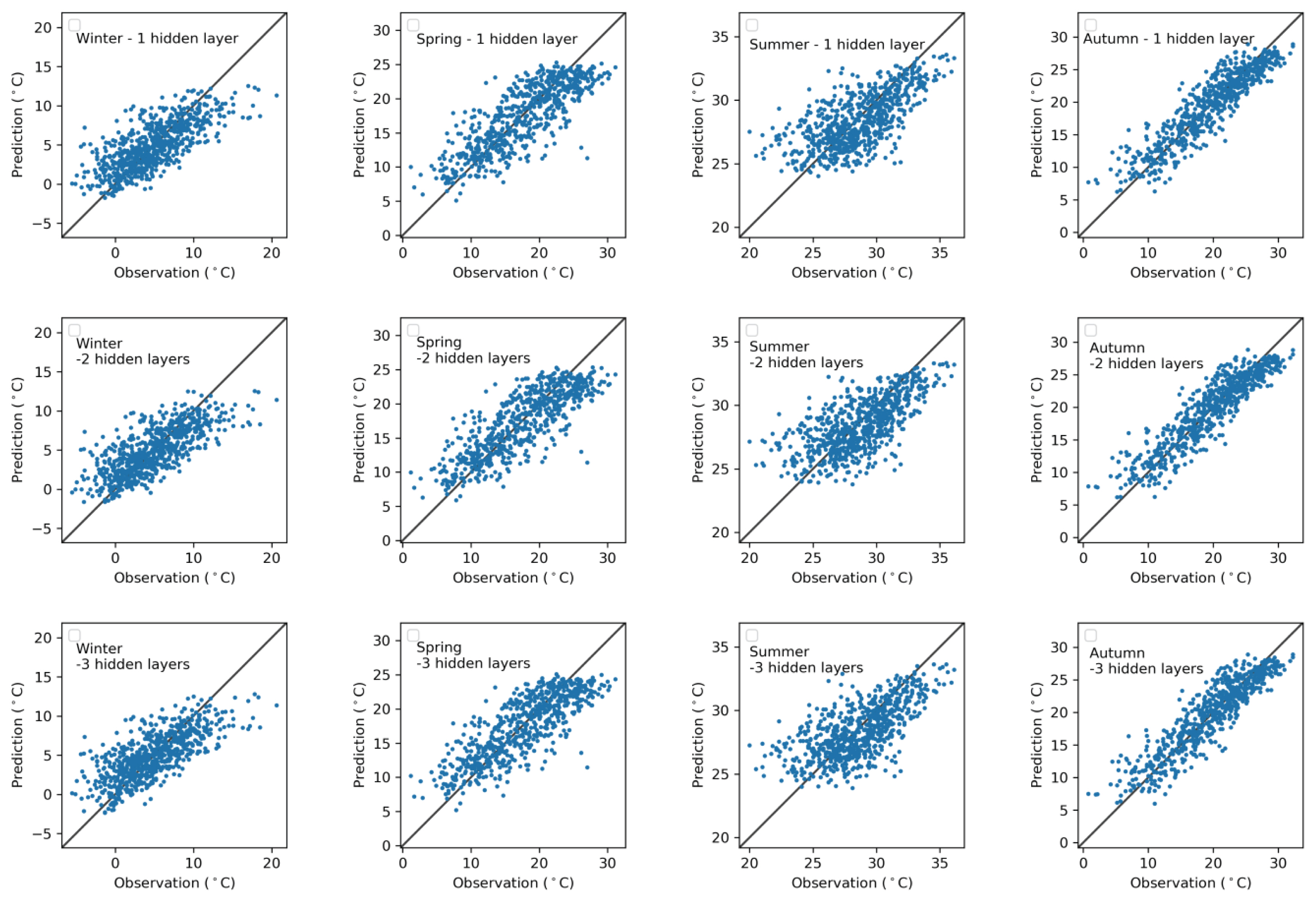
In this paper, we selected Gunsan station as a representative station to depict the scatter plot for maximum temperature prediction of the ANN model using one, two, and three hidden layers against the observed record (see Fig. 4). It can be seen from this figure that the model predicted quite well for one‐step (a day) ahead forecast in four seasons, especially the forecast values in the medium range of observed maximum temperature were relatively accurate. However, the figure showed that most of the low values were overestimated and high values were underestimated. For example, there is an overestimation for values above 15°C and underestimation for values below 0°C in winter. Furthermore, the predicted values deviated slightly from the observed values in spring and summer.
5. Conclusion
Estimating extreme temperature has a great significance as one of the major climate variables that is highly non‐linear, complex phenomenon affected by many climate and geographic variables. In this research, the neural network was used as a powerful tool in modeling nonlinear and undetermined procedures to predict maximum temperature in South Korea. We have forecasted one‐day‐ahead maximum temperature time series observed in five different stations of South Korea by using the artificial neural network.
The main aim of this multiple‐case study is to compare the performance of shallow (one‐hidden layer) networks with deep networks for forecasting extreme temperature. The optimal architecture of model is explored by using the genetic algorithm. Notably, in the five case studies described in this paper, the shallow ANN outperformed deep ANN with smaller errors. It has been empirically proven that the ANN with only three layers (one input, one hidden and one output) is sufficient for the maximum temperature forecast. The findings also suggest that more sophisticated networks do not necessarily provide better forecasts compared to simpler networks.
Acknowledgements
This work was supported by the National Research Foundation of Korea (NRF) grant funded by the Korean Government (MEST) (2018R1A2B6001799).


