Influence of Rain Gauge Density and Temporal Resolution on the Performance of Conditional Merging Method

Article information

J. Korean Soc. Hazard Mitig. 2019;19(6):41-51

Publication date (electronic) : 2019 November 30

doi : https://doi.org/10.9798/KOSHAM.2019.19.6.41

Duc Anh Dao ^*, Soohyun Kim ^**, Tae-Woong Kim ^***, Dongkyun Kim^,^****

^*Member, Doctor's Course, Department of Civil Engineering, Hongik University

^**Member, Doctor's Course, Department of Civil Engineering, Hongik University

^***Member, Professor, Department of Civil and Environmental Engineering, Hanyang University

^****Member, Associate Professor, Department of Civil Engineering, Hongik University

Corresponding Author, Member, Associate Professor, Department of Civil Engineering, Hongik University (Tel: +82-2-320-1613, Fax: +82-2-322-1244, E-mail: kim.dongkyun@hongik.ac.kr)

Received 2019 October 16; Revised 2019 October 16; Accepted 2019 October 31.

Abstract

본 연구는 in-situ 강우자료와 레이더자료를 병합하는 조건부 합성(CM)기법의 성능 평가를 목표로 한다. 합성방법은 다음 단계를 통해 처리된다. (1) 정규 크리깅(OK) 기법은 관측소와 레이더 기반 크리깅 강우장을 얻기 위해 적용한다. (2) 보정 강우장은 원래 레이더 강우장에서 레이더기반 크리깅 강우장의 차로 계산한다. (3) 합성강우량은 관측소기반 크리깅 강우장에 보정 강우장을 더하여 도출한다. 분석결과는 CM기반 강우장이 조사된 모든 33개의 10분 강우장 중 22개 사례에 대해 관측소기반 강우장보다 더 정확한 것으로 나타났다. CM 방법과 관측소기반 OK기법의 상관계수는 각각 0.63과 0.83 그리고 0.01과 0.74 사이 값을 보인다. 두 방법의 성능은 관측소 밀도가 높고 시간해상도가 낮을수록 향상되었다. OK기법의 성능은 관측소 밀도에 더 민감하고, CM 기법의 성능은 시간해상도에 더 민감한 것으로 나타났다. 또한, 기존 관측소 밀도가 100 km² 당 1개 일 때, 관측소를 추가하면 두 방법의 성능이 크게 향상되었다. 관측소 증가에 의한 강우량 측정 개선 정도는 관측소 개수가 100 km² 당 4개 이상에 도달할 시 효과가 미미한 것으로 나타났다.

Trans Abstract

This study aims to evaluate the performance of conditional merging (CM) technique to merge radar and in-situ rain gauge data. The merging method contains the following steps: (1) the ordinary kriging(OK) technique is applied to obtain the gauge-only and radar-only kriged rainfall fields; (2) the correction field is calculated by subtracting the radar-only kriged rainfall field from the original radar field; (3) the composite rainfall is derived by adding the correction field to the gauge-only kriged field. We investigated 33 10-min rainfall fields; there were 22 instances where the CM-based rainfall fields were more accurate than the gauge-only fields. The correlation coefficients of the CM and the gauge-only OK methods varied between 0.63 and 0.83, and 0.01 and 0.74 respectively. The performance of both methods improved with greater gauge density and coarser temporal resolution. Furthermore, the OK and CM techniques’performances were more sensitive to gauge density and temporal resolution respectively. We also found that the addition of gauge significantly improved the performance of both methods when the existing gauge density is approximately 1 gauge/100 km². However, this effect is absent when the density reaches 4 gauges/100 km².

Keywords: 정규 크리깅; 조건부 병합; 레이더; 우량계

Keywords: Ordinary Kriging; Conditional Merging; Radar; Rain Gauge

1. Introduction

The rainfall data with high spatial and temporal resolution are crucial for accurate hydrologic modelling (Kalinga and Gan, 2006;Cole and Moore, 2008; Li and Zhang, 2008; Langella et al., 2010; Li and Shao, 2010; Gebregiorgis and Hossain, 2012; Berne and Krajewski, 2013; Bhattacharya et al., 2013; Xu et al., 2013; Yao et al., 2014; Zhang et al., 2016).

In-situ gauge and weather radar are the two most widely applied measurement techniques to observe rainfall. The in-situ rain gauges provide accurate measurements at point locations, but its accuracy decreases with the decrease gauge spatial density especially when rainstorms have significant spatial variability (Hughes, 2006; Beesley et al., 2009; Renard et al., 2010; Kim et al., 2019). A variety of interpolation methods have been developed to produce the spatial rainfall estimates based on in-situ gauge data, including ordinary kriging (Bárdossy, 1993), kriging with external drift (Hudson and Wackernagel, 1994; Goovaerts, 2000), cokriging (Bárdossy and Lehmann, 1998; Lloyd, 2005), nearest neighbor (Isaaks and Srivastava, 1989), spline fitting techniques (Hutchinson, 1998). On the other hand, radar measurement can provide rainfall estimate over a large spatial coverage with high spatio-temporal resolution (Qi et al., 2013; Zhang et al., 2016). However, the radar rainfall data is subject to greater uncertainty compared to the in-situ gauge rainfall data because it infers the rainfall intensity from the microwave backscatter signal (Wilson and Brandes, 1979; Goudenhoofdt and Delobbe 2009; Shen et al., 2010; Wu and Zhai, 2012; Qin et al., 2014; Karbalaee et al., 2017).

The techniques of merging ground and radar data have been proposed to overcome the drawbacks of both measurement methods (Krajewski, 1987; Burlando et al., 1996; Schiemann et al., 2011; Pettazzi et al., 2012). The idea of merging the two different rainfall estimates was first proposed by Krajewski (1987). Then, the approach was further improved with various algorithms (Creutin et al., 1988; Seo, 1998; Sinclair and Pegram, 2005; Chumchean et al., 2006; Velasco-Forero et al., 2009; Berndt et al., 2014; Sideris et al., 2014). Haberlandt (2007) employed the kriging with external drift method to spatially interpolate the hourly rain gauge data using the drift information extracted from the radar data. Li and Shao (2010) developed a nonparametric kernel interpolation method to combine the rain gauge and TRMM satellite data, which does not rely on the stationarity assumption as kriging methods. The kriging with radar error method was developed by Ehret (2003), and it was called the Conditional Merging (CM) by Sinclair and Pegram (2005). The method adjusts the gauge-only kriged rainfall field using the information on the spatial structure of the rainstorms that is derived from the radar data.

The objective of this study is to evaluate the performance of the CM method. There have been various studies evaluating the performance of this technique (Haberlandt, 2007; Kim et al., 2007; Chappel et al., 2013; Baik et al., 2016; Sun et al., 2016; Chao et al., 2018). However, those studies used hourly and daily rainfall data, which do not meet the requirement of temporal resolution and cause the uncertainty in flood simulation in urban area (Rafieeinasab et al., 2015). In contrast, this study employed the gauge rainfall data with the temporal resolution of 10-minutes, which is commonly used in urban flood analysis. In addition, we can investigate the effect of temporal resolution on the performance of rainfall estimation in the range of sub-hourly timescales, which was not done in previous studies. The influence of gauge density on performance was also considered in this study.

2. Methodology

2.1 Study area and rainfall data

The study area is Seoul, the capital of Korea. The city is highly urbanized, covering an area of 605 km² with 239 sub-watersheds (Fig. 1). The study used 1-minute rainfall from 29 rain gauges (green dots in Fig. 1) and 10-minute temporal resolution radar provided by the Korea Meteorological Administration (KMA). The detail information of 29 stations is described in Table 1. The temporal periods investigated in this study is between 2010/09/21 12:30 and 2010/09/21 17:50 which totals up to 9,280 gauges measurements and 33 radar images. Fig. 2 shows the 10-minute hyetograph and the accumulated rainfall of the average areal rainfall over Seoul for the rainfall event period. The rain event was caused by the collision of the Siberian High and the North Pacific High, which caused localized rainfall with great spatial variability. The accumulated rainfall over the event period is the second highest in the record history of Seoul.

Fig. 1

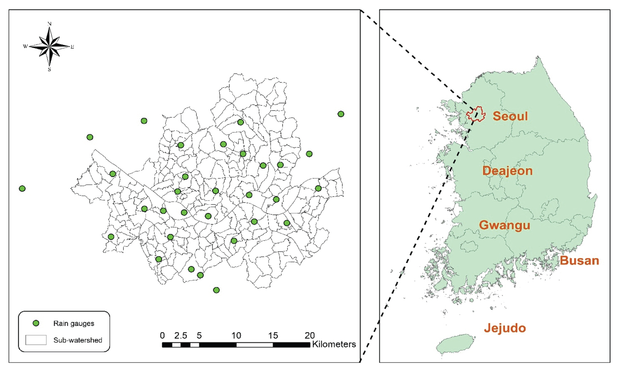
Location of Seoul City and Rain Gauge Network

Table 1

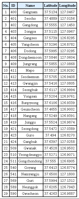
The Information of Gauge Stations

Fig. 2

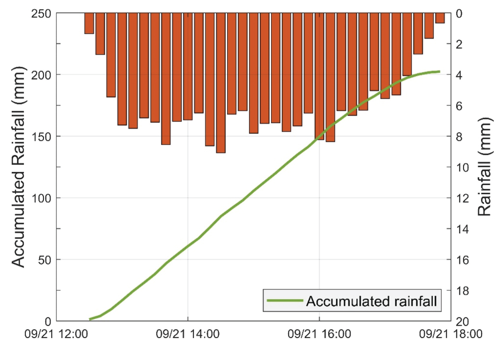
The 10-minute Hyetograph and the Accumulated Rainfall of the Event of the September 2010 that was Investigated in this Study

2.2 Conditional merging method

The conditional merging technique (Ehret, 2003; Sinclair and Pegram, 2005) assumes that the gauge provides the true source of spatial interpolation and the radar data provides auxiliary information on rainfall spatial variability to improve the accuracy (Goudenhoofdt and Delobbe, 2009; Rabiei and Haberlandt, 2015). The method has been proven to produce accurate spatial fields of various environmental variables (Sinclair and Pegram, 2005; Goudenhoofdt and Delobbe, 2009; Berndt et al., 2014; Baik et al., 2016; Kim et al., 2016).

Regarding to kriging method, it is assumed that a theoretical semivariogram model is to be fitted to an empirical one based on the normally distributed precipitation dataset. An appropriate estimate of the semivariogram value, γ^(h) , for point pairs separated by lag distance h is a measure representing the spatial variability of a regionalized variable z and is given by

(1) γ^(h)=12N(h)∑i=1N(h)[z(ui)-z(ui+h)]2

Where u_i and u_i + h refer point pairs with the distance of h, and N(h) is the number of point pairs with the same lag distance ; z(u_i) and z(u_i + h) indicate the observed variable at locations u_i and u_i + h, respectively, i is the number of data values. The set of estimates with each lag distance is designated as the empirical semivariogram which will be used to fit theoretical semivariogram by adopting a weighted least squares strategy to seek the best variogram parameters (Robinson and Metternicht, 2006). In this study, we used the isotropic exponential model (Eq. (2)) which was fitted to experimental variogram.

(2) γh=C0+C1[1-exp(-3ha)]

Here, a is range, C₁ the sill and C₀ the nugget effect.

Fig. 3 describes the CM technique applied in this study. This technique has the following procedures:

Fig. 3

The Process of the Conditional Merging

(a) One-minute ground-observed rainfall data is converted into 10-minute format to be synchronized with the measurement interval of the radar data. Then, gauge rainfall data were interpolated using Ordinary Kriging technique to obtain the gauge-only kriged rainfall field.

(b) Collect the radar rainfall data.

(c) The radar pixel values at the gauge locations were picked up and apply Ordinary Kriging technique to obtain the radar-only kriged rainfall field.

(d) Compute the correction field by subtracting the radar-only kriged rainfall field (c) from the original radar field (b).

(e) The composite rainfall was derived by adding correction field (d) to gauge-only kriged rainfall field (a).

2.3 Performance validation

The study used the leave-one-out cross-validation (CV) method to validate performance of two spatial interpolation method including the CM and the OK method (Schuurmans and Bierkens, 2007; Erdin, 2009; Kim et al., 2013, 2016; Kim et al., 2019). In this method, one of the rain gauges is assumed to be non-existent. Then, the remaining values are used to generate rainfall estimate at the point that was assumed non-existent. This set of process is repeated for all gauges. Lastly, the observed and the estimated values are compared.

2.4 Scenarios for gauge density and temporal resolution

The previous studies on the spatial interpolation method have concluded that the density of gauge network and temporal resolution are important to the performance of spatial interpolation (Krajewski, 1987; Goudenhoofdt and Delobbe, 2009; Berndt et al., 2014; Baik et al., 2016). This study analyzed this effect through 25 scenarios changing the of number of available gauges (6, 12, 18, 24, and 29 gauges) and temporal resolution (10, 20, 40, 60, and 80 minute).

In detail, given one case of gauge density, we create 5 scenarios of temporal resolution and it is applied for all case to generate totally 25 scenarios.

The network density scenarios were generated by randomly selecting the rain gauges, in which the scenario 1 represents to the use all available rain gauge data (Fig. 1). In 4 remaining cases, the number of gauges used to estimate rainfall was gradually reduced (Fig. 4).

Fig. 4

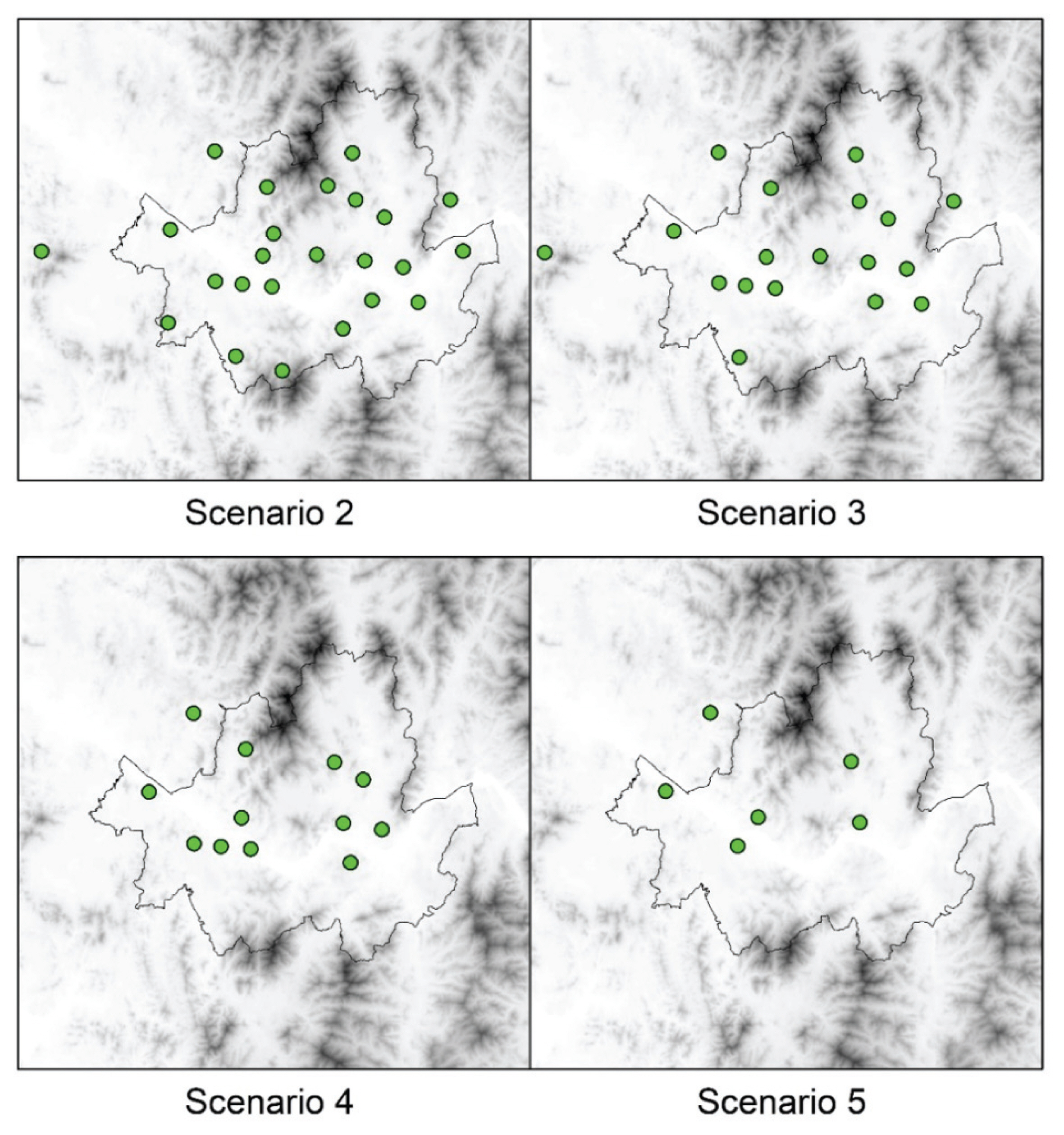
The Rain Gauges Density Scenarios. The Green Points Represent the Gauges Used to Estimate Rainfall

3. Results and discussions

3.1 The performance of conditional merging method

Fig. 5(a) compares the observed (x) and the estimated (y) rainfall produced by the OK and the CM method for time snapshot of 12:50 PM, September 21, 2010. The green stars and red circles represent the OK method and the CM method, respectively. For this specific time, the CM method showed the higher correlation coefficient (r=0.83) than the OK method (r=0.66).

Fig. 5

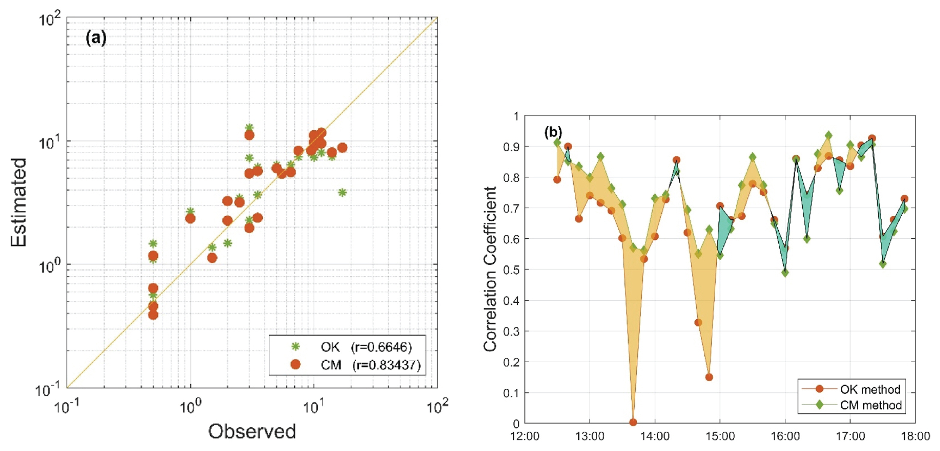
The Comparison Between CM and OK Technique in Terms of Correlation Coefficient

Fig. 5(b) compares the correlation coefficient for all 33 10-minute time steps investigated in this study. The green diamonds and red circles correspond to the CM and OK method, respectively. The orange polygon indicates the period that CM method outperforms the OK method, while the blue polygon indicates the opposite case. There are 22 times that CM method shows the greater correlation coefficient value compared to 11 times of the OK method. Moreover, the area of blue polygon is substantially smaller than that of orange polygon, indicating that the CM method remarkably improved the rainfall estimation.

3.2 The influence of gauge density and temporal resolution

Fig. 6 compares the correlation coefficient and the RMSE of the CM and the OK techniques varying with different gauge density values.

Fig. 6

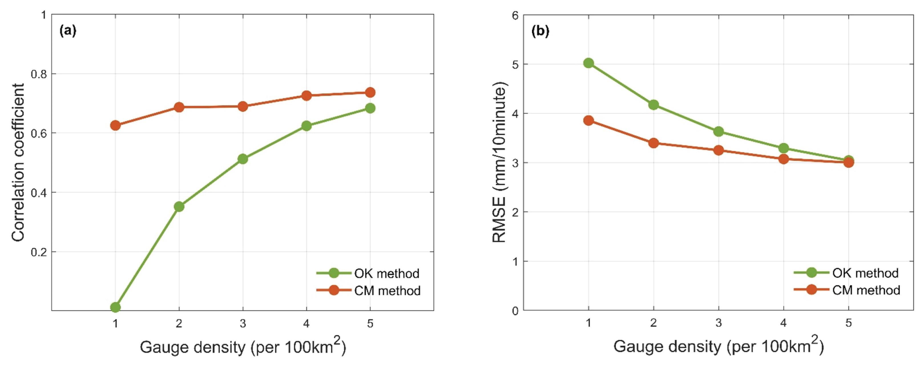
Average Performance of CM and OK Technique Over all Gauge Density Scenarios at a 10-minute Temporal Resolution

For both methods, the correlation coefficient value (r) increases with the increase of rain gauge density, while the RMSE value increases as density decreases. The OK method was more sensitive to the gauge density compared to the CM method. This is because the OK method relies only on the gauge measurements while the CM method uses both radar and gauge data. We also found that the influence of the gauge density does not increase dramatically when gauge density exceeds 4 gauges/100 km² for both techniques. The CM method shows the higher r value and lower RMSE value than the OK method for all 5 gauge density scenarios.

Fig. 7 compares the r and RMSE value varying with different temporal resolution of source rainfall data. The plots suggest that the accuracy of both methods increases with the increase of temporal resolution. The CM method showed greater performance for all 5 cases of rainfall temporal resolution.

Fig. 7

Average Performance of CM and OK Technique Over all Temporal Scenarios with Station Density of 100%

The Fig. 8 shows the r and the RMSE values varying with gauge density and temporal resolution. The color contours were generated by placing the r and RMSE values in the 2 dimensional space composed of gauge density and temporal resolution and spatially interpolating them.

Fig. 8

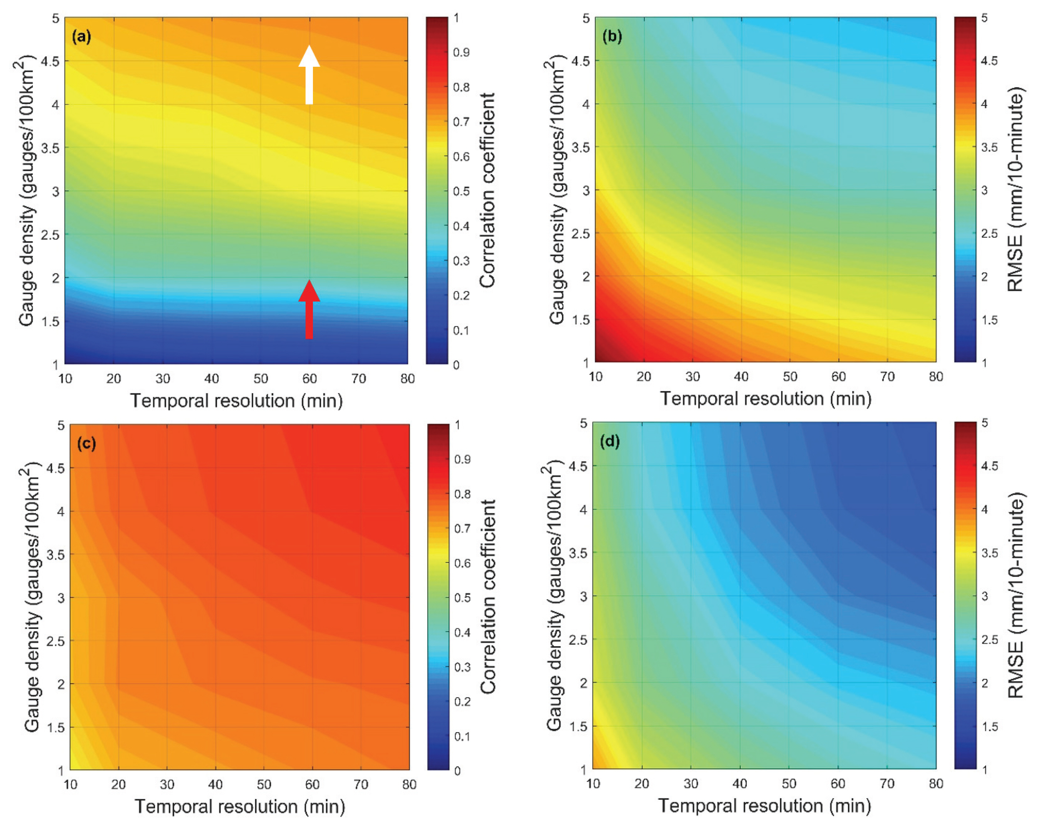
(a) The Correlation Coefficient and the (b) RMSE varying with temporal resolution and gauge density of the rainfall value estimated by the OK method. (c) The correlation coefficient and the (d) RMSE varying with temporal resolution and gauge density of the rainfall value estimated by the CM method.

In general, the r value increases as the increase of gauge density and accumulation time for both cases. Note that the areas in the contour plots with steep slope represent the abrupt performance change, which may provide a guideline on the minimum gauge density and the temporal resolution of the data to acquire a given degree of accuracy. For example, look at the red arrow in Fig. 8(a). The correlation coefficient at the starting and the ending point of the arrow correspond to the hourly rainfall estimation with the gauge density of 1.3 gauges/100 km² and 2 gauges/100 km². In this range, installation of only a few gauges can dramatically increase the accuracy of rainfall estimation. The white arrow, which has the same length as the red arrow suggests that the performance improvement would be minimal for the installation of additional gauges exceeding a given threshold of gauge density. The results also show that the CM method is more influenced by the temporal resolution compared to OK method.

4. Discussion

This study demonstrates that the CM method has strengthened the accuracy of rainfall simulation, which plays a major role in flood studies using hydrological modeling. We also found that increasing the number of gauge stations will improve the performance of methods investigated in study. However, this improvement degree is substantial when the station density is in the range of 1 to 4 gauges / 100 km². It helps decision makers to choose the optimal number of stations ensuring the accuracy of rainfall simulation with reasonable cost. Increasing the accumulation time also improves the accuracy of the CM method but reduces the applicability of its product. For example, for the study of urban flood, it requires the rainfall data with accumulation time of 15 minutes at least. Therefore, the consideration between improving the performance of CM method through increasing the accumulation time and applicability of the product should also be given.

5. Conclusions

The main objective of this study was to investigate the performance of conditional merging (CM) technique that combines the gauge and radar rainfall data varying with different in-situ gauge density and temporal resolution of input data. The control data for comparison was the rainfall field produced by the Ordinary Kriging (OK) technique that used only the in-situ gauge data. The leave-one-out cross validation method was used to quantify the performance of the CM and the OK method. The main finding of this study can be summarized as follows:

(1) The CM method showed the improved performance (greater r and smaller RMSE values) for all 25 scenarios of gauge densities and temporal resolutions.

(2) The performance of the CM and the OK method increased with the greater gauge density and coarser temporal resolution. The performance of the OK method was more sensitive to the gauge density than the CM method was. In contrast, temporal resolution has greater impact on the performance of CM method compared to OK method.

(3) The performance of both methods did not dramatically improve exceeding the gauge density of 4 gauges/ 100 km². Conversely, addition of only a few gauges can dramatically improve the rainfall estimation performance of both methods when the existing gauge density is very low (~ 1 gauge/100 km²).

Acknowledgements

This research was supported by a grant (MOIS-DP-2015-05) of Disaster Prediction and Mitigation Technology Development Program funded by Ministry of Interior and Safety (MOIS, Korea).

References

Baik J, Park J, Ryu D, Choi M. 2016;Geospatial blending to improve spatial mapping of precipitation with high spatial resolution by merging satellite-based and ground-based data. Hydrological Processes 30(16):2789–2803.

Bárdossy A. 1993. Stochastische modelle zur beschreibung der raum-zeitlichen variabilität des niederschlages Mitt. Inst. für Hydrologie und Wasserwirtschaft der Univ. Karlsruhe, Bd. 43, Karlsruhe:

Bádossy A, Lehmann W. 1998;Spatial distribution of soil moisture in a small catchment. Part 1: Geostatistical analysis. Journal of Hydrology 206(1–2):1–15.

Beesley C, Frost A, Zajaczkowski J. 2009. A comparison of the BAWAP and SILO spatially interpolated daily rainfall datasets. In : 18th World IMACS/MODSIM Congress. Cairns, Australia. p. 3886–3892.

Berndt C, Rabiei E, Haberlandt U. 2014;Geostatistical merging of rain gauge and radar data for high temporal resolutions and various station density scenarios. Journal of Hydrology 508:88–101.

Berne A, Krajewski WF. 2013;Radar for hydrology: Unfulfilled promise or unrecognized potential? Advances in Water Resources 51:357–366.

Bhattacharya A, Adhikari A, Maitra A. 2013;Multi-technique observations on precipitation and other related phenomena during cyclone aila at a tropical location. International Journal of Remote Sensing 34(6):1965–1980.

Burlando P, Montanari A, Ranzi R. 1996;Forecasting of storm rainfall by combined use of radar, rain gages and linear models. Atmospheric Research 42(1–4):199–216.

Chao L, Zhang K, Li Z, Zhu Y, Wang J, Yu Z. 2018;Geographically weighted regression based methods for merging satellite and gauge precipitation. Journal of Hydrology 558:275–289.

Chappell A, Renzullo LJ, Raupach TH, Haylock M. 2013;Evaluating geostatistical methods of blending satellite and gauge data to estimate near real-time daily rainfall for Australia. Journal of Hydrology 493:105–114.

Chumchean S, Sharma A, Seed A. 2006;An integrated approach to error correction for real-time radar-rainfall estimation. Journal of Atmospheric and Oceanic Technology 23(1):67–79.

Cole SJ, Moore RJ. 2008;Hydrological modelling using raingauge- and radar-based estimators of areal rainfall. Journal of Hydrology 358(3–4):159–181.

Creutin J, Delrieu G, Lebel T. 1988;Rain measurement by raingage-radar combination: A geostatistical approach. Journal of Atmospheric and Oceanic Technology 5(1):102–115.

Ehret U. 2003. Rainfall and flood nowcasting in small catchments using weather radar Hamburg, Germany: Institut für Wasserbau.

Erdin R. 2009. Combining rain gauge and radar measurements of a heavy precipitation event over Switzerland: Comparison of geostatistical methods and investigation of important influencing factors Zürich, Switzerland: Bundesamt für Meteorologie und Klimatologie.

Gebregiorgis AS, Hossain F. 2012;Understanding the dependence of satellite rainfall uncertainty on topography and climate for hydrologic model simulation. IEEE Transactions on Geoscience and Remote Sensing 51(1):704–718.

Goovaerts P. 2000;Geostatistical approaches for incorporating elevation into the spatial interpolation of rainfall. Journal of Hydrology 228(1–2):113–129.

Goudenhoofdt E, Delobbe L. 2009;Evaluation of radar-gauge merging methods for quantitative precipitation estimates. Hydrology and Earth System Sciences 13(2):195–203.

Haberlandt U. 2007;Geostatistical interpolation of hourly precipitation from rain gauges and radar for a large-scale extreme rainfall event. Journal of Hydrology 332(1–2):144–157.

Hudson G, Wackernagel H. 1994;Mapping temperature using kriging with external drift: Theory and an example from Scotland. International Journal of Climatology 14(1):77–91.

Hughes D. 2006;Comparison of satellite rainfall data with observations from gauging station networks. Journal of Hydrology 327(3–4):399–410.

Hutchinson MF. 1998;Interpolation of rainfall data with thin plate smoothing splines. Part I: Two dimensional smoothing of data with short range correlation. Journal of Geographic Information and Decision Analysis 2(2):139–151.

Isaaks EH, Srivastava RM. 1989. An introduction to applied geostatistics New York, USA: Oxford University Press.

Kalinga OA, Gan TY. 2006;Semi-distributed modelling of basin hydrology with radar and gauged precipitation. Hydrological Processes 20(17):3725–3746.

Karbalaee N, Hsu K, Sorooshian S, Braithwaite D. 2017;Bias adjustment of infrared-based rainfall estimation using passive microwave satellite rainfall data. Journal of Geophysical Research: Atmospheres 122(7):3859–3876.

Kim B, Hong J, Kim H, Choi K. 2007;Combining radar and rain gauge rainfall estimates for flood forecasting using conditional merging method. Journal of the Korean Society of Civil Engineers 27(3B):255–265.

Kim D, Lee J, Kim H, Choi M. 2016;Spatial composition of AMSR2 soil moisture products by conditional merging technique with ground soil moisture data. Stochastic Environmental Research and Risk Assessment 30(8):2109–2126.

Kim D, Olivera F, Cho H, Socolofsky SA. 2013;Regionalization of the modified Bartlett-Lewis rectangular pulse stochastic rainfall model. Terrestrial, Atmospheric & Oceanic Sciences 24(3):421–436.

Kim J, Lee J, Kim D, Kang B. 2019;The role of rainfall spatial variability in estimating areal reduction factors. Journal of Hydrology 568:416–426.

Krajewski WF. 1987;Cokriging radar-rainfall and rain gage data. Journal of Geophysical Research: Atmospheres 92(D8):9571–9580.

Langella G, Basile A, Bonfante A, Terribile F. 2010;High-resolution space–time rainfall analysis using integrated ANN inference systems. Journal of Hydrology 387(3–4):328–342.

Li M, Shao Q. 2010;An improved statistical approach to merge satellite rainfall estimates and raingauge data. Journal of Hydrology 385(1–4):51–64.

Li Z, Zhang K. 2008;Comparison of three GIS-based hydrological models. Journal of Hydrologic Engineering 13(5):364–370.

Lloyd C. 2005;Assessing the effect of integrating elevation data into the estimation of monthly precipitation in Great Britain. Journal of Hydrology 308(1–4):128–150.

Pettazzi A, Salsón S. 2012. Combining radar and rain gauges rainfall estimates using conditional merging: A case study. In : Proceedings of the Seventh European Conference on Radar in Meteorology and Hydrology, QPE (Quanitative Precipitation Estimation). p. 35.

Qi Y, Zhang J, Zhang P. 2013;A real-time automated convective and stratiform precipitation segregation algorithm in native radar coordinates. Quarterly Journal of the Royal Meteorological Society 139(677):2233–2240.

Qin Y, Chen Z, Shen Y, Zhang S, Shi R. 2014;Evaluation of satellite rainfall estimates over the Chinese mainland. Remote Sensing 6(11):11649–11672.

Rabiei E, Haberlandt U. 2015;Applying bias correction for merging rain gauge and radar data. Journal of Hydrology 522:544–557.

Rafieeinasab A, Norouzi A, Seo D, Nelson B. 2015;Improving high-resolution quantitative precipitation estimation via fusion of multiple radar-based precipitation products. Journal of Hydrology 531:320–336.

Renard B, Kavetski D, Kuczera G, Thyer M, Franks SW. 2010;Understanding predictive uncertainty in hydrologic modeling: The challenge of identifying input and structural errors. Water Resources Research 46(5):W05521. 10.1029/2009WR008328.

Robinson T, Metternicht G. 2006;Testing the performance of spatial interpolation techniques for mapping soil properties. Computers and Electronics in Agriculture 50(2):97–108.

Schuurmans J, Bierkens M. 2007;Effect of spatial distribution of daily rainfall on interior catchment response of a distributed hydrological model. Hydrology and Earth System Sciences 11(2):677–693.

Seo D. 1998;Real-time estimation of rainfall fields using radar rainfall and rain gage data. Journal of Hydrology 208(1–2):37–52.

Shen Y, Xiong A, Wang Y, Xie P. 2010;Performance of high-resolution satellite precipitation products over China. Journal of Geophysical Research: Atmospheres 115(D2):D02114. 10.1029/2009JD012097.

Sideris I, Gabella M, Erdin R, Germann U. 2014;Real-time radar–rain-gauge merging using spatio-temporal co-kriging with external drift in the alpine terrain of Switzerland. Quarterly Journal of the Royal Meteorological Society 140(680):1097–1111.

Sinclair S, Pegram G. 2005;Combining radar and rain gauge rainfall estimates using conditional merging. Atmospheric Science Letters 6(1):19–22.

Sun R, Yuan H, Liu X, Jiang X. 2016;Evaluation of the latest satellite–gauge precipitation products and their hydrologic applications over the Huaihe River basin. Journal of Hydrology 536:302–319.

Velasco-Forero CA, Sempere-Torres D, Cassiraga EF, Gómez-Hernández JJ. 2009;A non-parametric automatic blending methodology to estimate rainfall fields from rain gauge and radar data. Advances in Water Resources 32(7):986–1002.

Wilson JW, Brandes EA. 1979;Radar measurement of rainfall—A summary. Bulletin of the American Meteorological Society 60(9):1048–1060.

Wu L, Zhai P. 2012;Validation of daily precipitation from two high-resolution satellite precipitation datasets over the Tibetan Plateau and the regions to its east. Acta Meteorologica Sinica 26(6):735–745.

Xu H, Xu C, Chen H, Zhang Z, Li L. 2013;Assessing the influence of rain gauge density and distribution on hydrological model performance in a humid region of China. Journal of Hydrology 505:1–12.

Yao C, Zhang K, Yu Z, Li Z, Li Q. 2014;Improving the flood prediction capability of the Xinanjiang model in ungauged nested catchments by coupling it with the geomorphologic instantaneous unit hydrograph. Journal of Hydrology 517:1035–1048.

Zhang J, Howard K, Langston C, Kaney B, Qi Y, Tang L, et al. 2016;Multi-radar multi-sensor (MRMS) quantitative precipitation estimation: Initial operating capabilities. Bulletin of the American Meteorological Society 97(4):621–638.

No.	ID	Name	Latitude	Longitude
1	400	Gangnam	37.5134	127.0467
2	401	Seocho	37.4889	127.0156
3	402	Gangdong	37.5555	127.1450
4	403	Songpa	37.5115	127.0967
5	404	Gangseo	37.5739	126.8295
6	405	Yangcheon	37.5296	126.8782
7	406	Dodong	37.5995	127.0295
8	408	Dongdaemoon	37.5846	127.0604
9	409	Jungrang	37.5855	127.0868
10	411	Mapo	37.5517	126.9292
11	412	Seodaemun	37.5705	126.9408
12	413	Gwangjin	37.5416	127.0805
13	414	Seongbuk	37.6117	126.9994
14	415	Yongsan	37.5204	126.9761
15	416	Eunpyeong	37.6106	126.9339
16	417	Geumcheon	37.4655	126.9002
17	418	Hangang	37.5249	126.9391
18	419	Junggu	37.5524	126.9874
19	421	Seongdong	37.5472	127.0389
20	423	Guro	37.494	126.8270
21	424	Gangbuk	37.6397	127.0258
22	509	Gwanak	37.4528	126.9502
23	510	Yeongdeungpo	37.5271	126.9071
24	511	Gongchondong	37.555	126.6905
25	540	Goyang	37.6413	126.8774
26	541	Namyangju	37.6500	127.1800
27	569	Guri	37.5994	127.1312
28	589	Neunggok	37.6205	126.7943
29	590	Gwacheon	37.4263	126.9887