Evaluation of Key Issues for Converting Monthly WRAP Model to Daily WRAP Model

Article information

Abstract

Trans Abstract

1. Introduction

The Water Rights Analysis Package (WRAP) model based on monthly flows is a generalized river/reservoir development, management, control, allocation, and use focused on water use However, because the conventional WRAP model has a limitation to simulate the flood control reservoir operation, the sub-monthly WRAP model has been required. Accordingly, the expanded version of WRAP model, called as daily WRAP model, was developed. The daily WRAP model can perform computations at an interval of a day and provides additional features for simulating flood control operations, environmental instream flow requirements and so on (Wurbs and Hoffpauir, 2013). To simulate the daily WRAP model, the fundamental requirement prepare for the daily time input dataset. In particular, key modeling issues in the daily time step WRAP model simulation are the disaggregation of monthly naturalized flows into daily flows and then the integration of flood control reservoir operation into existing conservation reservoir modeling systems (i.e., calibration of routing parameters).

The WRAP model has been developed and applied to various hydrology areas and water resource-related projects. The application of the WRAP model in the Texas Water Availability Model (WAM) system is as follows: a monthly time-step input dataset development (HDR Engineering, Inc. 2001a, 2001b); application of the conventional WRAP model (Salazar and Wurbs, 2004; Wurbs, 2006; Wurbs et al., 2012); and application of the conventional and expanded versions of the WRAP model (Wurbs and Kim, 2011; Kim and Wurbs, 2011a, 2011b; Kim, 2011, 2012, 2014, 2015).

In this study, disaggregation of monthly streamflow based on daily pattern method proposed by Wurbs and Hoffpauir (2013) that includes and routing paramenter calibration based on reach length are used. In detail, two kinds of key factors in the daily time step WRAP model were assessed as follows. First, daily naturalized flows developed by the U.S. Army of Corps of Engineers (USACE) Forth Worth District were utilized as daily flow patterns and then disaggregate monthly inflows of the Brazos River Authority Condensed (BRAC) datasets to daily inflows. Second, routing parameters computation was performed for normal and flood flows.

2. Case Study and WRAP Model

The Brazos River Basin has a total area of 115,565 km² shown in Fig. 1. The average annual temperature varies from 16°C in the high plains to 21°C in the Gulf Marshes and Prairies. The mean annual precipitation varies from 483 mm in the upper basin which lies in the High Plains, to 1,143 mm in the lower basin in the Gulf Coast region. The BRAC dataset (Kim and Wurbs, 2011a) consisting of 14 reservoirs and water rights related to reservoirs and control points were considered and utilized in this study (Kim and Wurbs, 2011c; Wurbs and Hoffpauir, 2013).

Fig. 1.

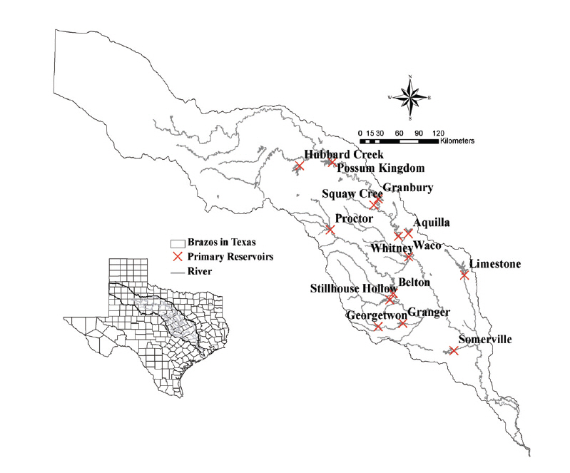
The Brazos River Basin, Texas, USA

The conventional WRAP model based on a monthly time step is composed of a set used for executing WRAP programs within Microsoft operation system. The SIM program is used for simulating water allocation for a system of rivers, reservoirs, and water use. The HYD program is for developing data for monthly naturalized stream flow and reservoir net evaporation-precipitation depth. The TABLES program is used for organizing the simulation results according to a user-defined format and for exporting the data to Microsoft Excel or HEC-DSSVue. The expanded version of the WRAP model is based on a daily time step and consists of the SIMD program for sub-monthly time step simulation, flow forecasting, routing, and flood control simulation features; the DAY program for daily or other sub-monthly time-interval flows from monthly naturalized flow synthesis and routing parameter calibration; the SALT program for salinity modeling; and the conventional WRAP model (Wurbs, 2015a, 2015b; Kim and Wurbs, 2011c; Wurbs and Hoffpauir, 2013).

3. Methodologies

Disaggregation refers to the process of subdividing monthly time intervals into daily or sub-monthly time intervals. The alternative methods for dividing monthly naturalized flow volumes between time steps within each month were outlined by Wurbs and Hoffpauir (2013). The monthly values of input variables are disaggregated within SIMD into sub-monthly amounts as follows. 1) Naturalized flows are provided directly as input data or disaggregated monthly naturalized flows. 2) Diversion and hydropower targets are uniformly distributed over the sub-monthly time intervals. Alternatively, options later limit targets to a specified number of days or allow targets to vary across a month depending on daily water availability. 3) Instream flow targets are uniformly distributed over the sub-monthly time intervals. Alternatively, an option limits targets to a specified number of days. 4) Net evaporation depths or constant inflows are uniformly distributed over the sub-monthly time intervals. In other words, the monthly quantities except monthly streamflows are simply divided by the number of days in the month to obtain the daily amounts. The daily unregulated (naturalized) flows from 1940 through 1997 from the USACE Southwestern Division Reservoir System Simulation Model (SUPER) dataset are used as daily flow patterns to disaggregate the BRAC monthly naturalized flows, which are the focus of this study. Even though the flow pattern method has a limitation that does not mimic the long-term non-stationary shift in flow (e.g. climate change) at each control point, the method can be used one of methods to generate the daily flow with monthly flow when daily flows are not gaged. Table 1 shows the availability of SUPER daily flow in BRAC datasets. 25 SUPER model gage IDs are matched to BRAC control points. The matched 25 control points are shown in bold in Fig. 2.

Table 1.

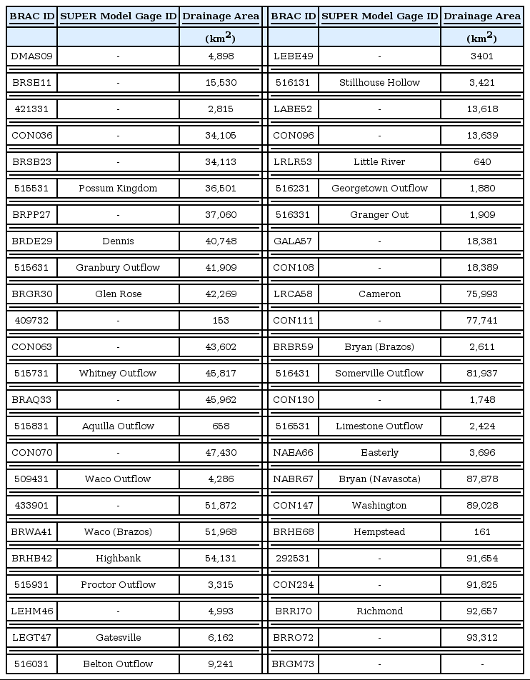
Availability of SUPER Model Daily Naturalized Flows in BRAC Dataset

Fig. 2.

Schematic of Available SUPER Model Daily Naturalized Flows in BRAC Datasets in the Brazos River Basin, Texas

3.1 Extension of Daily Flow Pattern for Hydrologic Simulation Periods

The hydrological simulation periods of BRAC flow cover 1900 through 2007, while those of the SUPER daily naturalized flow cover 1939 through 1997. The flow patterns for 1900 to 1938 and 1998 to 2007 of missing periods were developed from SUPER model daily naturalized flow for 1939 to 1997 at 25 control points. Although mean flows, median flows, or any other exceedance frequency flows could be used, the mean daily flows on each day are proposed as being reasonably likely flows. The flow volume in the 59 years is determined using SUPER model flows at a particular control point for 1939 to 1997. For example, at each control point, the January 1 flow volume averaged for 59 years in the SUPER model flow dataset for 1939 to 1997 is determined. Average flows are determined for each of the 365 days. The resulting set of 365 flow volumes for January 1 through December 31 are repeated for each of the 39 years from 1900 to 1938 and 10 years from 1998 to 2007. Fig. 3 shows the average daily flow pattern at 515531 (Possum Kingdom) and BRRI70 (Richmond), which has available flows located at the most and lowest control points, respectively.

Fig. 3.

Averaged Daily Flow Pattern at Most Upstream and Downstream Control Points

The plotted average daily flows sustain their patterns even though each day during the 59 years is averaged. These averaged dataset are used to apply the daily flow pattern for the two periods of BRAC flow (1900 to 1938 and 1998 to 2007). Table 1 lists the drainage areas at 48 control points. The unknown daily flow pattern at 23 control points illustrated in this table can be acquired by transferring known flow patterns at 25 control points based on the drainage area ratio method (Hirsch, 1979).

3.2 Transferring Daily Naturalized Flows Patterns at 25 Control Points to 23 Other Control Points

The 48 control points of the condensed datasets are divided into two groups. In the first group, daily flow patterns from the daily naturalized flows of the SUPER model are available for 1990 to 2007 for 25 of the control points. For the second group, daily flow patterns are not available for the other 23 control points, so the patterns for 1900 to 2007 at each of the 23 control points are transferred based on the SUPER daily naturalized flow at one of the 25 control points within the DAY program while considering lag time.

Lag times are computed using a linear cross-correlation method in the DAY program between gaged inflow and gaged outflow. The results of lag time calibration are listed in Table 2. The values for lag time may be transferred to other reaches based on reach lengths. In this study, the lag time of intermediate control points are assumed to be zero if the computed lag time is zero or one between two control points in the SUPER model dataset and one or more intermediated control points in the BRAC datasets are located on the reach. If the computed lag time is more than 2 between two control points included in the SUPER model dataset and one or more intermediate control points in the BRAC datasets, the value of the lag time is estimated based on reach lengths. After calibration, only two lag times between 515931 and LEHM46 and between LEHM46 and LEGT47 are one, while lag times for those remaining between upstream and downstream control points are zero.

Table 2.

Calibration Results of Lag Time Using SUPER Daily Naturalized Flows

The 23 unknown-flow control points are listed in Table 3 along with the relationship with known-flow control points. The flow pattern of the daily naturalized flow at each of the 23 unknown flow control points were related by ratios of drainage area at one selected known-flow control point. In most cases, the unknown-flow and known-flow control points are located on the same stream. In some cases, known-flow control points in adjacent watersheds were selected for transferring at a particular unknown-flow control point. For 8 of the unknown-flow control points, flow patterns are transferred from the same control points that are used for distributing primary control point flows to secondary control points. In 15 cases, different control points are used to transfer daily naturalized flow at unknown-flow control points.

Table 3.

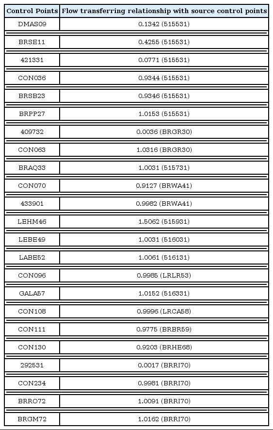
Relationships for Transferring 1900-2007 Flow Patterns for 23 Control Points

3.3 Routing Parameters Calibration

Calibration of routing parameters is another key task for adjusting daily flows between two control points. In this study, the direct Muskingum parameter calibration option embedded in the WRAP model are considered at the first stage. Its methods consists of computation of travel time (K) and weighting coefficient (X). Eq. (1) reflect the fundamental definition of parameters K and X in Muskingum method.

(1) ST=K[ITX+OT(1.0-X)]

Where, S_T is storage volume at the end of day T, I_T is inflow volume during day T, and O_T is outflow volume during day T

In other words, the direct Muskingum parameters calibration method in the WRAP model computes K for assumed values of X raning from 0.0 to 0.5. that increase 0.5 or 1.0 in each simulation step. Finally. the linear correlation coefficient (R) is used as criteria to determine best K with the fixed X. However, the poor R coefficients calibrated between two control points indicate the direct method can not be used in the daily WRAP model. Accordingly, two assumptions are used as follows: first, K can be estimated based on proportioning travel time. Because distance can serve as a surrogate for travel time in proportioning K to reaches of varying length; and second, the value of X is assumed to be zero at every control point. Also, normal stream velocity and flood stream velocity are assumed to be 24.4km/day and 64.4km/day to determine K in each flow. The reason is that flow velocities are greater and travel times shorter for flood flows compared to normal flows (Wurbs and Hoffpauir, 2013). Table 4 shows the results of K calibrated with the assumptions.

Table 4.

Muskingum Routing Parameter K for Normal and Flood Flow

4. Summary and Conclusion

In this study, daily flow patterns were utilized for disaggregating BRAC inflow and routing parameters based on length are computed. The SUPER model daily unregulated (naturalized) flows from 1939 to 1997 at 25 of the 37 control points developed by the Fort Worth District of the USACE were used to develop daily flow patterns for disaggregating BRAC monthly inflows. The mean values of the daily naturalized flow for 1939 to 1997 at 25 control points were used as the flow pattern for 1900 to 1939 and 1998 to 2007. These daily flow patterns were distributed to the other 23 ungaged control points. The lag times at 48 control points of the BRAC dataset were computed based on the distance of the reaches with consideration of the lag time computed using the SUPER daily naturalized flow. The Muskingum routing parameters K at 35 control points were also computed based on the distance of the reaches with the assumption that normal stream velocity and flood stream velocity are 15 miles/day (0.92 ft/s) and 40 miles/day (2.44 ft/s), respectively. Based on these results, validation of daily flow pattern application to BRAC for inflows from 1900 to 2007 can be performed in future studies, and Muskingum routing parameters can be calibrated using optimization functions embedded in the DAY or SIMD programs. This study provides beneficial information for an expanded version of WRAP model simulation to water rights permit projects and water resource management.

Article information Continued